Gran-DEM Documentation is a centralized knowledge base designed to help users understand, manage, and utilize all features of the Gran-DEM platform. It provides comprehensive guides, setup instructions, best practices, troubleshooting resources, and technical references to ensure a smooth and efficient user experience.
1.
Introduction
The Gran-DEM particle flow simulator is a commercial particle flow DISCRETE ELEMENT METHOD (DEM) application that can be used to simulate particle flow in any type of pre-designed 3-D domain. This 3-D domain can be a mesh file (.msh) imported into the Gran-DEM application. The Gran-DEM application set-up (version 1.0) can be licensed and downloaded from (gran-dem.com) and installed. The procedure to do this is provided hereby;
The application can next be started from the start menu. The Gran-DEM particle flow simulator is operated using a tailor developed User interface for easy formulation and set-up. The Gran-DEM UI opens immediately after starting it from the start menu. The UI design consists of 3 vertical panes LEFT (red), MIDDLE (green) and RIGHT (blue) and a horizontal TOP (orange) pane that can be seen in Fig 1.1. The UI set-up consists of 7 main functionalities organized sequentially in the left most pane of the UI. These main functionalities are SELECT MODEL, MATERIALS, SYSTEM, PARTICLE MODEL, PARTICLE INJECTION, FLUID FLOWSOLVER, BOUNDARY CONDITIONS, MONITORS, USER DEFINED FUNCTIONS, EXECUTE AND PARAVIEW VISUALIZATION.
Fig. 1.1: UI layout design and its main subdivided functionalities.
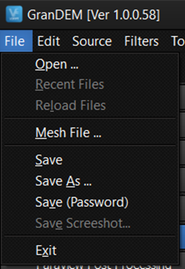
When any of the above main functionalities is selected the sub-selections for these appear in the middle pane. The right large pane is used for visualization. The top pane (orange) consists of File, Edit, Source, Filters, Tools and Help that are described later in Section 8.1. In the following sections various aspects of the UI operations are discussed sequentially.
2.
Select Model
2.1
Description and theory
The Select Model dialog is the starting point for configuring a simulation in GranDEM. It allows users to activate the Continuous Fluid Phase (CFD), the Discrete Particle Phase (DEM), and define the coupling mechanisms between them. Depending on the selected options, GranDEM can perform pure CFD simulations, pure DEM simulations, or fully coupled CFD-DEM simulations with momentum, heat, and mass transfer.
The LnE multiphase CFD simulator is a multipurpose tool for carrying out both Lagrangian (granular) and Eulerian (Fluid) flow simulations in various flexible combinations. The Eulerian (fluid) flow modelling is done by using the coupled pressure-velocity model that involves fundamentally the continuity Equation and Navier Stokes Equation solved on a 3D grid domain.
Within the CFD framework this is also called the SIMPLE algorithm that stands for Semi-Implicit Method for Pressure Linked Equation proposed by Spalding and Patankar (1978). Typically, most commercial CFD solvers for unstructured grid domains use the finite volume method where the pressure and velocities are collocated at cell centre positions. However, the formulation used here is a staggered grid approach where the scalars, like pressure is defined at cell centre and vectors like velocity is defined at face centre (or staggered) position. The Single phase Eulerian can be solved with or without heat transfer (energy balance) and multi-component mass transfer.
The Lagrangian particle flow modelling uses the Discrete Element Method (DEM) for treating collision mechanism. The Eulerian fluid flowsolver can be coupled 2-ways for momentum transfer or exchange with discrete particle phase or DEM. Additionally if heat and mass transfer with the fluid phase is to be initiated then it can be done.
Another feature of Gran-dem is its DEM can be coupled with external software such as ANSYS FLUENT fluid flowsolver. This coupling can be done for all 3 aspects i.e. momentum, heat and mass transfer.
Figure 2.1
Figure 2.1: Select Model dialog showing CFD, DEM, coupling options and external solver exchange paths.
Table 2.1 Field Description
No.
Field
Description
①
Continuous Fluid Phase
Enables or disables the Eulerian fluid flow solver.
②
Heat Transfer
Activates the energy equation for thermal simulations.
③
Multi Component Mass Transfer
Enables transport of multiple chemical species.
④
Discrete Particle Phase
Enables the DEM particle solver.
⑤
Coupling Momentum Transfer
Transfers momentum between particles and fluid.
⑥
Coupling Heat Transfer
Allows thermal energy exchange between phases.
⑦
Coupling Mass Transfer
Allows species exchange between particles and fluid.
⑧
Path to Exchange (Write)
Directory where GranDEM writes coupling files for an external CFD solver.
⑨
Path to Exchange (Read)
Directory from which GranDEM reads updated CFD data.
① Continuous Fluid Phase
Purpose
Activates the Eulerian fluid solver.
Usage
Enable this option whenever fluid flow calculations are required.
Typical Applications
Air flow
Water flow
Gas flow
Fluidized beds
Pneumatic conveying
② Heat Transfer
Purpose
Solves the energy equation and predicts temperature distribution.
Enable When
Cooling analysis
Heating processes
Furnaces
Heat exchangers
Drying simulations
③ Multi Component Mass Transfer
Purpose
Models transport of multiple chemical species.
Applications
Drying
Evaporation
Gas diffusion
Chemical reactors
④ Discrete Particle Phase
Purpose
Activates the DEM solver.
Applications
Granular flow
Powder mixing
Conveyors
Crushers
Hoppers
⑤ Coupling Momentum Transfer
Purpose
Transfers drag and reaction forces between particles and fluid.
Use When
Both CFD and DEM are enabled.
⑥ Coupling Heat Transfer
Allows thermal energy exchange between particles and the surrounding fluid.
Typical examples include particle cooling, heating, combustion, and drying.
⑦ Coupling Mass Transfer
Allows evaporation, condensation, moisture transport, and chemical species exchange between particles and the fluid.
⑧ Path to Exchange (Write)
Specifies the directory where GranDEM exports coupling data for an external CFD solver.
⑨ Path to Exchange (Read)
Specifies the directory from which GranDEM imports updated CFD solution files.
Typical Simulation Configurations
CFD Only
Continuous Fluid Phase ✔
DEM ✘
DEM Only
Continuous Fluid Phase ✘
DEM ✔
CFD-DEM Coupling
Continuous Fluid Phase ✔
DEM ✔
Momentum Transfer ✔
Fully Coupled Multiphysics
CFD ✔
DEM ✔
Momentum ✔
Heat ✔
Mass ✔
2.2
Setting up
On the Main UI ‘Select Model’ setting from the left pane. Under the continuous phase drop down menu election for the Eulerian fluid flow method can be made or set off.
If Fixed field, single phase Eulerian or single phase External (Fluent) is selected the user can switch on the fluid heat transfer and/or mass transfer model.
If the DEM method in discrete particle phase is switched on the user can choose to couple ‘Momentum transfer’, ‘Heat transfer’ and/or ‘Mass transfer’ with the fluid phase (Eulerian) using the switches below it (Refer Fig. 2.1).
If the user wants to use this feature ‘momentum transfer’ is mandatory but the remaining 2 can be chosen.
If single phase External (Fluent) has been selected in the continuous phase the user should add the path to the exchange directory at the bottom of the left pane Fig. 2.1. This is needed to connect with ANSYS FLUENT and exchange coupling data.
3.
Material properties
3.1
Description and theory
The flow behaviour of materials is fundamentally characterised by their physical properties. Therefore, material properties of Eulerian fluids (liquid or gas) and Lagrangian particles (liquid or solid) during CFD flow simulations are extremely important while simulating system flow behavior. The Eulerian Fluid phase can be single component or multiple component. Depending on the choices made in select model for species transport components can be added to Eulerian fluids and their physical properties entered the check boxes.
Similarly, the particles properties are added into in a separate section on left pane depending on if DEM has been selected in ‘Select Model’. The particle flow dramatically affect phenomena such as segregation, wettability, heat and mass transfer, etc within process systems. The fundamental properties of particle material needed for DEM simulations are density, viscosity, thermal conductivity, species diffusivity and heat capacity. Properties like viscosity are relevant only when discrete particles are actually droplets or particles are wet. Similarly, properties like thermal conductivity are relevant when heat transfer is considered or simulations are non-isothermal.
3.2
Setting up
On the Main UI, select ‘Material Properties’ from the left pane. This causes the component materials adding additional tabs in the middle pane to appear. This consists of the buttons ‘Add component’ and ‘Delete component’.
Using the ‘Add component’ button new components can be added successively which appear one below the other as ‘Component 1’, ‘Component 2’, etc. (Fig. 3.1).
Under each component, check boxes are provided for adding the ‘Component name’ and ‘Molecular Weight’ of the component. It also has a switch called ‘volatile’ indicating if the component is volatile or not and a button called ‘physical properties.
The ‘volatile’ switch is switch on for components that can vaporise from the Lagrangian or discrete particles into the surroundings. It is typically switched on for components like water that can vaporize and leave the discrete phase. But for components like fertilizers, aluminum, iron oxide, etc. that do not typically vaporize during DEM simulations it need not be switched on.
When the ‘physical properties’ button is clicked (see Fig. 3.2) it opens a tab to enter in the properties ‘density, viscosity, thermal conductivity, species diffusivity and heat capacity’. Note that as discrete particles are in either solid or liquid phase these properties that are to be entered are in one of these phases.
If the volatile switch is on, all the above mentioned (point 5) properties are duplicated to add properties in gaseous state as well. This is essential to evaluate process parameters such as vaporization rate, vapor pressure, etc.
It also provides for a thermodynamic stability factor (Rm[GU1] ) that gives the stability coefficient between the volatile component and non-volatile component.
Fig. 3.1: The component setting in the middle pane.
1. Add / Delete Component
Add Component creates a new material component (Component 1, Component 2, Component 3, etc.).
Delete Component removes the selected material component.
Multiple components can be defined for multi-component particles.
2. Component Name Enter the name of the material component.
Examples
Water
Sand
Coal
Iron Oxide
Fertilizer
Com-01
This name is used throughout the simulation and in thermodynamic calculations.
3. Molecular Weight Specify the molecular weight of the component.
Typical units:
kg/kmol (or g/mol depending on the software convention)
Examples:
Water = 18
Oxygen = 32
Nitrogen = 28
The molecular weight is used during species transport, evaporation, diffusion, and thermodynamic calculations.
4. Volatile Switch Enable this switch if the material can evaporate or vaporize.
ON
Water
Alcohol
Solvents
OFF
Sand
Iron
Alumina
Fertilizer
When enabled, GranDEM additionally considers gaseous-phase properties for the component and computes vaporization-related processes.
5. Physical Properties Click Physical Properties to define the material properties of the component.
Typical properties include:
Density
Dynamic Viscosity
Thermal Conductivity
Specific Heat Capacity
Species Diffusivity
If the component is marked as Volatile, additional gas-phase properties are also required.
6. Thermodynamic Equilibrium (RM Factors) This table defines the RM (Relative Miscibility / Thermodynamic Stability) Factors between volatile and non-volatile components.
Columns:
ID
RM Factor(s)
RM Value
These values are used during evaporation and multi-component mass transfer calculations.
Example:
RM Factor
Description
Water / Fertilizer
Stability factor
Water / Salt
Stability factor
Water / Sugar
Stability factor
7. RM Value Enter the numerical RM coefficient for each component pair.
This coefficient influences:
Phase equilibrium
Evaporation behaviour
Mass transfer calculations
Multi-component thermodynamics
8. Eulerian Fluid Properties This section defines the gas/fluid components used in the Eulerian CFD solver.
Similar to the particle material section, users can:
Add/Delete gas components
Specify gas name
Enter molecular weight
Define gas physical properties
These components are used for CFD calculations involving airflow, species transport, heat transfer, and coupled DEM-CFD simulations.
9. Gas Physical Properties Click Physical Properties to define the fluid properties for the selected gas component.
Typical gas properties include:
Density
Dynamic Viscosity
Thermal Conductivity
Specific Heat Capacity
Species Diffusivity
These properties are required for solving:
Navier-Stokes equations
Heat transfer
Mass transfer
Species transport
Fig. 3.2: Insertion of physical properties of individual component without (left) and with volatility (right)
Description of Fields
1. Component Name
Displays the name of the material component whose properties are being edited.
This helps identify the currently selected material component.
2. Density (kg/m³)
Specifies the material density.
Density determines the particle mass and directly influences:
Particle weight
Inertia
Momentum
Collision behaviour
Packing characteristics
Typical values
Material
Density (kg/m³)
Water
1000
Sand
2650
Glass
2500
Steel
7850
3. Viscosity (kg/ms)
Specifies the dynamic viscosity of the material.
Viscosity represents the internal resistance of the material to deformation or flow.
Higher viscosity results in:
Greater resistance to motion
Reduced particle mobility
Increased damping during flow
Typical values
Material
Dynamic Viscosity
Water
0.001 kg/ms
Oil
Higher than water
4. Thermal Conductivity (W/mK)
Defines the ability of the material to conduct heat.
This property is used when Heat Transfer is enabled.
Higher thermal conductivity allows heat to transfer more rapidly through the material.
Typical values
Material
Thermal Conductivity (W/mK)
Water
0.6
Steel
45–60
Copper
~400
5. Species Diffusivity (kg/s)
Specifies the diffusion property of the material species.
This parameter is used during:
Multi-component mass transfer
Species transport
Evaporation
CFD-DEM coupled simulations
Higher diffusivity results in faster species transport between phases.
6. Heat Capacity (J/kgK)
Defines the specific heat capacity of the material.
This property determines the amount of heat required to raise the temperature of one kilogram of material by one Kelvin.
It is used in:
Energy balance calculations
Heating and cooling processes
Thermal simulations
Typical values
Material
Heat Capacity (J/kgK)
Water
4186
Steel
~500
Aluminium
~900
Volatile Materials
If the Volatile option is enabled for a component in the Material Properties window, the Physical Properties dialog is extended to include additional properties for the gaseous phase.
In this case, users must define both:
Liquid/Solid Phase Properties
Density
Viscosity
Thermal Conductivity
Species Diffusivity
Heat Capacity
Gas Phase Properties
Gas Density
Gas Viscosity
Gas Thermal Conductivity
Gas Species Diffusivity
Gas Heat Capacity
These additional properties are required for accurately modelling:
Evaporation
Vaporization
Heat transfer
Mass transfer
DEM-CFD coupled simulations
4.
System
4.1
Description and theory
The main functionality of system motion is of relevance when DEM simulations need to be performed where the domain motion is also simulated alongside DEM particles. The domain motion here can be of two types namely; vibrational motion and rotational motion. Under this functionality the system domain or Eulerian grid consisting of nodes, cells and faces position changes dynamically with time. This begins from an original position and periodically depending on the type of motion returns to the original position.
In case of vibrational motion, the entire domain including the Eulerian grid nodes, cells and faces move in a vibrational form with an amplitude and a time constant. The vibrational motion also needs to be set with vibrational direction.
In case of rotational motion, the domain including the Eulerian grid nodes, cells and faces move about a position axis at a given fixed rotational speed.
4.2
Setting up
The System Motion module is used to define external motion fields acting on the simulation domain. These motion fields include Gravity, Vibration, and Rotation, allowing users to simulate stationary, vibrating, and rotating systems.
To access this module, select System Motion from the left navigation pane. The middle pane displays three tabs:
Gravity
Vibration
Rotation
Fig 4.1: System motion model selection showing the gravity tab.
Gravity
The Gravity tab is used to define the gravitational acceleration acting on particles and fluids during the simulation. Users can enable or disable gravity, specify its magnitude, and define the direction of the gravitational field.
Gravity is applied uniformly throughout the computational domain.
Description of Fields
1. Gravity Enable Switch
The On/Off switch enables or disables gravity during the simulation.
ON
Gravity is included in the governing equations.
Particles experience gravitational acceleration.
Fluid body forces due to gravity are also considered (when CFD is enabled).
OFF
Gravity is ignored.
Useful for zero-gravity or microgravity simulations.
2. Gravity Magnitude (m/s²)
This field specifies the magnitude of gravitational acceleration.
which represents the standard gravitational acceleration on Earth.
Users may specify different values to simulate other environments.
Examples
Environment
Gravity (m/s²)
Earth
9.81
Moon
1.62
Mars
3.71
Zero Gravity
0.0
3. Direction Definition Method
GranDEM provides two methods for specifying the gravity direction.
Vector
Defines gravity using Cartesian vector components.
This method is suitable when the direction is known in terms of X, Y, and Z coordinates.
Angle
Defines gravity using angular coordinates.
This option is useful when gravity direction is easier to express as an angle rather than individual vector components.
4. Direction Components
When Vector mode is selected, the gravity direction is defined using three Cartesian components.
gX
Gravity component along the X-axis.
gY
Gravity component along the Y-axis.
gZ
Gravity component along the Z-axis.
Example
For gravity acting vertically downward in the negative Z direction:
Component
Value
gX
0
gY
0
gZ
-1
5. Unit Vector
The entered gravity direction is automatically treated as a unit vector.
The software internally normalizes the vector to ensure that only the direction is used while the specified gravity magnitude determines the acceleration.
6. Clear Button
The Clear button resets all direction component fields.
This allows users to quickly define a new gravity direction without manually deleting the existing values.
Working Principle
During simulation, GranDEM computes the gravitational force acting on each particle according to:
Fg=mg\mathbf{F_g}=m\mathbf{g}Fg=mg
where:
Fg = gravitational force (N)
m = particle mass (kg)
g = gravitational acceleration vector (m/s²)
The gravity vector is obtained from the user-defined magnitude and direction entered in the Gravity tab.
Applications
The Gravity module can be used to simulate:
Particle settling
Hopper discharge
Powder handling
Granular flow
Conveyor systems
Rotating drums
Fluidized beds
Sedimentation processes
DEM-CFD coupled simulations
Vibration
The Vibration tab is used to apply translational vibration to the simulation domain. This feature enables users to simulate systems where particles or fluids are subjected to periodic oscillatory motion, such as vibrating feeders, sieves, conveyors, compaction equipment, and mixing devices.
To use vibration, enable the On/Off switch and specify the vibration amplitude and time constant. During the simulation, the prescribed vibration is applied uniformly to the entire computational domain.
Fig 4.2: System motion model selection showing the vibration tab.
Description of Fields
1. Vibration Enable Switch
The On/Off switch enables or disables vibration during the simulation.
ON
Vibration is applied to the simulation domain.
Particle motion is influenced by the specified vibration parameters.
Suitable for modelling vibrating equipment and oscillatory motion.
OFF
No vibration is applied.
Particles move only under the influence of other forces such as gravity, contact forces, drag, and external loads.
2. Amplitude (m)
The Amplitude field specifies the maximum displacement of the vibrating system from its equilibrium position.
A larger amplitude produces greater displacement during each vibration cycle.
Typical examples:
Equipment
Typical Amplitude
Laboratory shaker
0.001–0.005 m
Vibrating feeder
0.002–0.010 m
Industrial screen
0.005–0.020 m
3. Time Constant (s)
The Time Constant defines the characteristic time associated with the vibration motion.
It controls how rapidly the vibration evolves with time and influences the transient response of the system.
Smaller values produce a faster response, while larger values result in a more gradual variation of the vibration.
Rotation
The Rotation tab is used to apply rotational motion to the simulation domain. This feature is particularly useful for modelling equipment such as rotating drums, tumblers, mixers, ball mills, rotary kilns, centrifuges, and rotating reactors.
When enabled, the simulation domain rotates about a user-defined axis passing through a specified point in space. Users can define the rotational speed, the direction of the rotation axis, and the position through which the axis passes.
Fig 4.3: System motion model selection showing the rotation tab.
Description of Fields
1. Rotation Enable Switch
The On/Off switch enables or disables rotational motion during the simulation.
ON
Rotational motion is applied to the computational domain.
Particles experience centrifugal and Coriolis effects depending on the rotational speed.
Suitable for rotating machinery and mixing applications.
OFF
No rotational motion is applied.
The simulation behaves as a stationary system unless other motion models are enabled.
2. Angular Speed (rps)
The Angular Speed field specifies the rotational speed of the system.
Higher angular speed increases the rotational velocity and consequently the centrifugal forces acting on the particles.
Typical examples:
Equipment
Angular Speed
Rotary Drum
0.1 – 2 rps
Ball Mill
1 – 5 rps
Centrifuge
10 – 100 rps
3. Axis (Unit Vector)
The Axis section defines the direction of the rotational axis using a unit vector.
The axis direction is specified by three Cartesian components.
X (m)
Defines the X-component of the rotation axis.
Y (m)
Defines the Y-component of the rotation axis.
Z (m)
Defines the Z-component of the rotation axis.
Example
For a drum rotating about the global Z-axis:
Component
Value
X
0
Y
0
Z
1
For rotation about the X-axis:
Component
Value
X
1
Y
0
Z
0
The entered values are automatically normalized internally to form a unit vector, ensuring that only the direction of the axis is considered.
4. Position
The Position section specifies a point through which the rotation axis passes.
The coordinates are entered in the global coordinate system.
X (m)
X-coordinate of the rotation axis.
Y (m)
Y-coordinate of the rotation axis.
Z (m)
Z-coordinate of the rotation axis.
Example
If the rotation axis passes through the origin:
Coordinate
Value
X
0
Y
0
Z
0
5. Clear Button
The Clear button resets all axis and position fields.
This allows users to quickly redefine the rotation axis without manually clearing each input box.
Working Principle
When rotational motion is enabled, GranDEM rotates the computational domain about the user-defined axis at the specified angular speed.
The rotation is completely defined by three parameters:
Angular Speed
Rotation Axis
Rotation Position
During the simulation, particles experience additional inertial effects associated with rotational motion, including:
Centrifugal force
Coriolis force (where applicable)
Rotational acceleration
These effects significantly influence particle trajectories, mixing behaviour, and material transport.
5.
Particle Models
5.1
Description and theory
The Discrete element method-based particle tracking is governed by Newton’s law of motion. The dynamic motion of any particle ‘a’, defined vectorially in a 3-D space by position vector ‘ra’ and mass ‘ma’, is determined by the sum of the forces acting on the particle. This balance is provided hereby in Eq. 3.1;
(3.1)
Where; \(F_G\) is the gravity force, \(F_C\) is the contact collision force and \(F_D\) is the drag force acting on the particle.
5.1.1
Gravity force
Gravity defines the natural influence of gravitation acting on the particle mass. It is given by Eq. (3.2):
(3.2)
Where; \(\vec{g}\) is the gravitational force vector defined at the center of mass of particle.
5.1.2
Collision force
Collision force is the summation of all direct contact collision forces experienced by the particle. The collision forces are treated by the soft sphere approach where a spring-dashpot method is applied. Therefore, any given particle ‘a’ can be simultaneously in collision with multiple particles ‘b’. Thus. the total collision force acting on any particle ‘a’ is sum of collision force with all contact particles ‘b’ in its contact space given by;
(3.3)
Where, \(F_{ab} \) is the contact force due to collision between any particle ‘a’ and ‘b’. This individual force defined by the spring-dashpot method is given by;
(3.4)
Where; \(k_n\) is the normal spring stiffness and \( \eta_n \) is the normal restitution coefficient. \( \overrightarrow{n_{ab}} \) and \( \overrightarrow{v_{ab}} \) are the positional unit normal vector and relative velocity between given particles ‘a’ and ‘b’, respectively. \( \delta_n \) is the prevailing contact overlap between the two particles. The normal overlap is given by;
(3.5)
Where, \(\vec{r}_a\) and \(\vec{r}_b\) represent the position vector for the colliding particles and \(\vec{r}_a\) and \(\vec{r}_b\) are the radii of respective particles.
5.1.3
Interphase drag force
The drag force is the force acting on particles due to fluid phase (gas or liquid) flowing around it. It is essentially the momentum transferred by the fluid phase due to friction when flowing passed the surface of the particle. This force typically can be modelled through a one way or a two-way coupling between the Lagrangian DEM phase and Eulerian fluid phase on a fixed grid. In the one way coupling only the particle phase drag is considered but in a two way coupling the drag force encountered by the fluid phase is also considered. The drag force acting on individual particle is given by;
(3.6)
Where; \(\beta_a\) is the drag coefficient, \(\vec{v_p}\) is the particle velocity vector and \(\vec{u_p}\) is the fluid velocity defined by the Eulerian grid mapped at the particle location.
5.2
Setting up
The Collision Force tab is used to define the contact force model governing interactions between discrete particles during DEM simulations. These parameters determine how particles behave when they come into contact with one another or with solid boundaries.
GranDEM uses the Cundall–Strack Contact Model, one of the most widely adopted soft-sphere DEM contact models. This model represents the contact between particles using normal and tangential springs, friction, and damping to simulate realistic collision behaviour.
Fig. 5.1:Particle Model window showing the Collision Force tab.
Description of Fields
1. Collision Force Enable Switch
The On/Off switch enables or disables the collision force model.
ON
Particle-particle and particle-wall contact forces are calculated.
DEM collision mechanics are activated.
Required for most granular flow simulations.
OFF
Contact forces are ignored.
Particles pass through one another without physical interaction.
Mainly intended for testing or specialised simulations.
2. Autoset
The Autoset option automatically computes suitable collision parameters based on the specified particle material properties.
When enabled, GranDEM estimates recommended values for:
Normal restitution
Tangential restitution
Spring stiffness
Tangential spring stiffness
Friction coefficients
This feature helps users quickly initialise simulations with physically reasonable parameters.
3. Cundall–Strack Model
GranDEM employs the Cundall–Strack soft-sphere contact model, in which contacting particles are represented by elastic springs and frictional sliders.
The model computes:
Normal elastic force
Tangential elastic force
Sliding friction
Rolling resistance
Energy dissipation during impacts
Contact Model Parameters
4. Normal Restitution (Norm.Res.)
The Normal Restitution Coefficient defines the elasticity of collisions in the direction normal to the contact surface.
Higher values cause particles to rebound more strongly after impact.
5. Tangential Restitution (Tang.Res.)
The Tangential Restitution Coefficient controls the recovery of tangential motion after contact.
Lower values produce greater damping of tangential motion during collisions.
6. Spring Stiffness (Spr.Stiff.)
The Spring Stiffness defines the normal contact stiffness between particles.
It controls how much two particles deform during collision.
Higher stiffness values result in:
Smaller particle overlap
Shorter collision duration
Increased numerical stiffness
Lower values permit greater overlap and softer collisions.
7. Tangential Spring Stiffness (T Spr.Stiff.)
The Tangential Spring Stiffness specifies the stiffness of the tangential contact spring.
This parameter influences:
Tangential force development
Sliding behaviour
Particle rolling characteristics
8. Frictional Coefficient (μ_f)
The Friction Coefficient controls sliding friction between contacting surfaces.
Higher values:
Increase resistance to sliding
Reduce particle mobility
Improve particle interlocking
Lower values allow particles to slide more freely.
9. Rolling Friction Coefficient
The Rolling Friction Coefficient defines the resistance to particle rolling.
Higher rolling friction:
Reduces rolling motion
Produces more stable particle packing
Better represents irregular particle shapes
Granulation Parameter
10. Coalescence Threshold
The Coalescence Threshold specifies the minimum condition required for two colliding particles to merge (coalesce) during granulation simulations.
This parameter is primarily used in simulations involving:
Wet granulation
Pellet formation
Agglomeration
Powder processing
Pharmaceutical manufacturing
For DEM simulations that do not involve particle growth or agglomeration, this value can generally be left at its default setting.
Working Principle
During each simulation time step, GranDEM detects contacts between particles and computes the interaction forces using the Cundall–Strack contact model. The collision behaviour is governed by:
These parameters collectively determine how particles collide, rebound, slide, roll, dissipate energy, and, where applicable, merge into larger agglomerates.
Drag Force
The Drag Force model is used when particles interact with a surrounding fluid such as air, water, or gas. As particles move through the fluid, the fluid exerts a resistance force called drag force, which opposes the particle motion.
GranDEM provides several well-established drag force correlations from the scientific literature. The appropriate drag law should be selected based on the flow regime, Reynolds number, particle concentration, and application.
Fig. 5.2: Particle Model – Drag Force
① Drag Force Enable Switch
Purpose
Enables or disables drag force calculations.
Options
On – Fluid drag force is included in the DEM calculations.
Off – No drag force is applied to particles.
Recommendation
Enable this option whenever a fluid phase (air, gas, or liquid) interacts with particles.
② Drag Law Selection
This drop-down list allows the user to select the mathematical correlation used to calculate drag force.
Available models include:
Grace et al.
Schiller and Naumann
Ergun and Wen & Yu (1952)
Beetstra et al. (2007)
Tang et al. (2014)
Drag Force-6
Drag Force-7
Drag Force-8
Each model has been developed for different particle-fluid systems and operating conditions.
Available Drag Models
Grace et al.
Suitable for:
Fluidized beds
Gas-solid systems
Dense particle suspensions
Provides accurate drag predictions across a wide range of particle Reynolds numbers.
Schiller and Naumann
One of the most widely used drag correlations.
Recommended for:
Single particle motion
Dilute suspensions
Low to moderate Reynolds numbers
Commonly used in CFD-DEM simulations.
Ergun and Wen & Yu (1952)
Designed primarily for:
Packed beds
Dense particle assemblies
Fluidization calculations
Combines the Ergun equation with the Wen-Yu correlation to model drag over different solid volume fractions.
Beetstra et al. (2007)
Recommended for:
Dense particulate flows
CFD-DEM coupling
Gas-solid fluidized beds
Accounts for particle interactions in concentrated suspensions.
Tang et al. (2014)
Suitable for:
High solid volume fraction flows
Advanced multiphase simulations
Improved drag prediction in dense systems
Provides enhanced accuracy for modern DEM-CFD simulations.
Drag Force-6
Custom drag model available within GranDEM.
May be used for specialized research applications requiring alternate drag formulations.
Drag Force-7
Additional empirical drag correlation provided for advanced simulations.
Useful for validating different drag models against experimental data.
Drag Force-8
Alternative drag model intended for specialized particle-fluid interaction studies.
Users should select this model when recommended by project requirements or validation studies.
Selecting the Appropriate Drag Model
Simulation Type
Recommended Model
Single particle in air
Schiller and Naumann
Packed bed
Ergun and Wen & Yu
Fluidized bed
Grace et al.
Dense CFD-DEM simulation
Beetstra et al.
High concentration multiphase flow
Tang et al.
Research / Validation studies
Drag Force-6, 7, or 8
Notes
Drag force calculations are only meaningful when a continuous fluid phase is enabled.
The selected drag law significantly affects particle velocity, residence time, pressure drop, and fluid-particle momentum exchange.
Different drag models are optimized for different flow regimes. Users should choose the model appropriate for their application and, where possible, validate simulation results against experimental data or published literature.
6.
Injection Initialization
6.1
Description and theory
The injection of particles into the domain is set up in this functionality. Here a flexible injection system has been provided where user is able to choose from a variety of types of injection depending on requirement. There are 4 main types of injections that can be defined. They are;
Injection type 1: Specific point injection
Injection type 2: Cell centre fixed point injection
Injection type 3: Fixed square grid ordered injection
Injection type 4: Feed channel injection
PARTICLE INJECTION (FL_INJ):
6.1.1
Injection type 1: Specific point injection:
This is a completely flexible injection option provided where individual independent injection points can be defined as needed by the user. Each injection point is specified with basic variables like particle diameter, number of particles per parcel, parcel diameter, X, Y, Z position point in 3D space, X, Y, Z injection velocity in 3D space, Temperature and material composition. Besides each injection is also set with single or multiple injection. Single injection entails only 1 injection is made at time t=0.0s.
If multiple injection option is chosen the user needs to additionally specify mass flow rate and its dependent variable time constant. This leads to a continuous injection of particle at a fixed time interval space. This injection is also defined in terms of mass flow rate for the given particle injection. The start and end time for injection is also defined.
6.1.2
Injection type 2: Cell centre fixed point injection:
Injection points are created at the cell centre positions of all the Eulerian grid in the system. This setting requires basic variables specified as particle diameter, number of particles per parcel, parcel diameter, X, Y, Z position point in 3D space, mean injection velocity in 3D space, Temperature and material composition. The direction of injection here is always set in the gravity direction. These variables are set for all particles injected at all cell center positions. Besides, the injection is also set with single or multiple injection. Single injection entails only 1 injection is made at time t=0.0s.
If multiple injection option is chosen the user needs to additionally specify mass flow rate and its dependent variable time constant. This leads to a continuous injection of particle at a fixed time interval space. This injection is also defined in terms of mass flow rate for the given particle injection. The start and end time for injection is also defined. This injection type is typically used for filling up domain system with particles.
6.1.3
Injection type 3: Fixed square grid ordered injection:
Injection points are created in a fixed square grid. This setting involves minimum and maximum positions in X,Y,Z direction and particle pitch that needs to be provided. Here the minimum and maximum can be seen as a cutoff limit in the Eulerian grid as shown in Fig. 6.1. Using this info a square grid of injection points is generated where distance between particles in each direction is the pitch. The other variables provided as usual from previous are particle diameter, number of particles per parcel, parcel diameter, X, Y, Z injection velocity in 3D space, Temperature and material composition. These variables are set for all particles injected at the square grid positions. Besides, the injection is also set with single or multiple injection. Single injection entails only 1 injection is made at time t=0.0s.
Fig 6.1: Schematic showing minimum and maximum limit in an euilerian grid for limiting injection points.
If multiple injection option is chosen the user needs to additionally specify mass flow rate and its dependent variable time constant. This leads to a continuous injection of particle at a fixed time interval space. This injection is also defined in terms of mass flow rate for the given particle injection. The start and end time for injection is also defined. This injection type is typically used for filling up domain system with desired amount of particles.
6.1.4
Injection type 4: Feed channel injection:
This is a special injection type where a channel feed type of injection can be defined. The injection type requires to be set with a mass flow rate, particle injection velocity and position. Using this information concentric rings of injection points are created for particulate injection. Fig. 6.2 shows a schematic of an example arranged injection points. The size of the ring depends on the mass flow rate and the pitch provided by the user. The other variables provided as usual from previous are particle diameter, number of particles per parcel, parcel diameter, X, Y, Z injection velocity in 3D space, Temperature and material composition. These variables are set for all particles injected at the square grid positions.
Besides, the injection is also set with single or multiple injection. Single injection entails only 1 injection is made at time t=0.0s. If multiple injection option is chosen the user needs to additionally specify mass flow rate and its dependent variable time constant. This leads to a continuous injection of particle at a fixed time interval space. This injection is also defined in terms of mass flow rate for the given particle injection. The start and end time for injection is also defined. This injection type is typically used for filling up domain system with particles.
Fig 6.2: Feed stream channel injection arrangement in a ring form.
6.2
Setting up:
6.1 Injection Initialization – Specific Point Injection
The Specific Point Injection method is used to introduce particles into the computational domain from one or more user-defined locations. Each injection point represents a particle source where particles are generated with specified physical properties, initial velocity, temperature, and composition.
This injection method is suitable for simulations involving:
Spray nozzles
Powder feeders
Material discharge points
Hopper outlets
Granular injection into reactors
Particle dosing systems
The user can define multiple independent injection locations, each having its own particle properties and operating conditions.
Fig. 5.1: Specific Point Injection Settings
1. Specific Point (Enable)
Enables or disables the Specific Point Injection model.
Yes – Specific Point Injection is activated.
No – This injection model is ignored during simulation.
2. Number of Injection
Specifies the total number of independent injection points that will be created.
Example:
1 → Single injection location
5 → Five independent injection sources
3. Add Injections
Creates the specified number of injection entries.
After clicking this button, individual injection configurations become available.
4. Select Injection
Displays the list of all previously created injections.
The user can select an injection for editing or reviewing its properties.
Example:
Injection 1
Injection 2
Injection 3
5. Save
Stores all modifications made to the currently selected injection.
Changes are not permanently saved until this button is pressed.
6. Delete
Removes the selected injection definition from the project.
Deleting an injection permanently removes all associated settings.
Injection Parameters
7. Injection Name
A unique user-defined name used to identify the injection.
Examples:
Feed Inlet
Nozzle 1
Powder Source
Hopper Outlet
8. Particle Diameter (m)
Defines the diameter of an individual particle.
Unit:
metre (m)
Particle diameter influences:
Collision behaviour
Drag force
Packing characteristics
Heat transfer
Mass transfer
9. Parcel Diameter (m)
Defines the diameter of the computational parcel.
A parcel represents a collection of identical particles.
Parcel injection reduces computational cost for simulations involving millions of particles.
10. Number of Particles per Parcel
Specifies how many real particles are represented by a single computational parcel.
means
One computational parcel equals one physical particle.
Larger values are useful for large-scale industrial simulations.
Injection Position
The coordinates define the particle release location.
11. X (m)
X-coordinate of the injection point.
12. Y (m)
Y-coordinate of the injection point.
13. Z (m)
Z-coordinate of the injection point.
Together, these coordinates specify the exact particle injection location within the computational domain.
Initial Velocity
These fields specify the initial velocity of injected particles.
14. Vx (m/s)
Initial velocity along the X-direction.
15. Vy (m/s)
Initial velocity along the Y-direction.
16. Vz (m/s)
Initial velocity along the Z-direction.
These velocity components determine the particle trajectory immediately after injection.
Thermal Conditions
17. Temperature Unit
Allows selection of the temperature unit.
Typical options include:
Degree Celsius (°C)
Kelvin (K)
18. Temperature
Specifies the initial particle temperature at the moment of injection.
This parameter is required when heat transfer simulations are enabled.
Composition Mass Fraction
The lower table specifies the chemical composition of injected particles.
Each component previously defined in Material Properties appears automatically.
19. Component ID
Unique identifier of the material component.
20. Component Name
Displays the material name.
Example:
Water
Fertilizer
Sand
Iron Ore
21. Mass Fraction
Specifies the fraction of each component present within the injected particle.
The total mass fraction of all components must satisfy:
∑iYi=1\sum_i Y_i = 1i∑Yi=1
where:
YiY_iYi = Mass fraction of component i
Example:
Component
Mass Fraction
Water
0.20
Fertilizer
0.80
Total = 1.00
Injection Mode
22. Single / Multiple
Determines how the injection points are interpreted.
Single
A single particle source is used.
Suitable for:
Single nozzle
Hopper outlet
One inlet
Multiple
Allows several independent injection sources within the same simulation.
Useful for:
Multiple spray nozzles
Multi-port injectors
Distributed feeding systems
Multiple inlet locations
Notes
Every injection point can have independent particle size, velocity, temperature, and composition.
Position coordinates should lie within the computational domain.
The sum of all component mass fractions must equal 1.0.
When heat transfer is enabled, particle temperature should be specified.
Multiple injection sources can be configured to simulate complex industrial feeding systems.
Parcel-based injection significantly reduces computational cost while preserving the physical mass flow rate.
6.2 Injection Initialization – Cell Center Injection
The Cell Center Injection method is used to initialize particles uniformly within a specified three-dimensional region of the computational domain. Unlike the Specific Point Injection, where particles are released from one or more fixed locations, Cell Center Injection automatically generates particles at the center of each computational cell contained within the user-defined bounding box.
This injection method is particularly useful for simulations where particles are initially distributed throughout a volume rather than entering through an inlet.
Typical applications include:
Fluidized bed initialization
Packed bed generation
Bulk powder storage
Sediment bed formation
Initial particle distribution in reactors
Particle settling simulations
Fig. 6.2: Cell Center Injection settings.
Description of Fields
1. Cell Center Injection
The On/Off switch enables or disables the Cell Center Injection model.
ON
Particles are generated automatically at the center of every computational cell within the specified region.
OFF
Cell Center Injection is ignored during the simulation.
2. Save
Saves the current Cell Center Injection settings.
Any changes made to the injection parameters should be saved before running the simulation.
Particle Properties
3. Particle Diameter (m)
Specifies the diameter of each injected particle.
The particle diameter influences:
Particle mass
Collision behaviour
Drag force
Heat transfer
Packing density
4. Number of Particles per Parcel
Specifies the number of physical particles represented by one computational parcel.
indicates that one parcel represents one physical particle.
Using larger parcel sizes reduces computational cost while maintaining the desired mass loading.
5. Parcel Diameter (m)
Defines the effective diameter of the computational parcel.
Parcel-based injection allows efficient simulation of systems containing millions of particles.
Injection Region (Points)
The injection region is defined by a three-dimensional rectangular bounding box.
Particles are generated only inside this region.
6. Xmin (m)
Minimum X-coordinate of the injection region.
7. Xmax (m)
Maximum X-coordinate of the injection region.
8. Ymin (m)
Minimum Y-coordinate of the injection region.
9. Ymax (m)
Maximum Y-coordinate of the injection region.
10. Zmin (m)
Minimum Z-coordinate of the injection region.
11. Zmax (m)
Maximum Z-coordinate of the injection region.
Together, the six coordinates define the three-dimensional volume in which particles are initialized.
For example:
Coordinate
Value
Xmin
0.0
Xmax
0.10
Ymin
0.0
Ymax
0.05
Zmin
0.0
Zmax
0.20
This creates a rectangular region measuring 0.10 × 0.05 × 0.20 m.
Thermal Properties
12. Temperature Unit
Selects the unit of temperature.
Typical options include:
Degree Celsius (°C)
Kelvin (K)
13. Temperature
Specifies the initial temperature of the injected particles.
This field is required when heat transfer calculations are enabled.
Injection Velocity
14. Vm
Specifies the initial magnitude of particle velocity.
Unlike Specific Point Injection, where velocity is entered as separate Vx, Vy, and Vz components, Cell Center Injection uses a single velocity magnitude (Vm) that is applied uniformly to all initialized particles.
Typical values:
Application
Vm
Static packed bed
0 m/s
Slow feeding
0.1–1 m/s
Pneumatic conveying
5–20 m/s
Composition Mass Fraction
The lower table specifies the composition of the injected particles.
All material components defined under Material Properties are automatically listed.
15. Component ID
Unique identifier of each material component.
16. Component Name
Displays the name of each material component.
Examples:
Water
Sand
Fertilizer
Iron Ore
17. Mass Fraction
Specifies the mass fraction of each component in the injected particle.
The sum of all component mass fractions must satisfy:
∑iYi=1\sum_i Y_i = 1i∑Yi=1
Example:
Component
Mass Fraction
Water
0.30
Sand
0.70
Total = 1.00
Working Principle
When Cell Center Injection is enabled, GranDEM identifies all computational cells whose centers lie within the user-defined bounding box. A particle or computational parcel is then initialized at the center of each selected cell using the specified particle diameter, parcel size, temperature, velocity, and composition.
This approach provides a uniform initial particle distribution throughout the selected region and is particularly suitable for simulations that begin with a pre-filled particle bed rather than particles entering from a discrete inlet.
Notes
The injection region must lie entirely within the computational domain.
The total mass fraction of all components should equal 1.0.
Set Vm = 0 m/s when initializing a stationary particle bed.
Cell Center Injection generates particles based on the computational mesh, ensuring a uniform spatial distribution.
Larger parcel sizes can significantly reduce computational time for large-scale industrial simulations.
The Fixed Grid Injection method is used to inject particles from a uniformly spaced grid of predefined locations within a specified three-dimensional region. Unlike Cell Center Injection, where particles are automatically placed at the computational cell centers, Fixed Grid Injection generates particles at fixed intervals (grid spacing) defined by the user.
This method is particularly useful for creating controlled and evenly distributed particle injections over a specified volume or surface.
Typical applications include:
Uniform particle distribution
Spray nozzle arrays
Multiple feed points
Powder bed generation
Bulk material loading
Reactor initialization
Granulation studies
Fig. 6.3: Fixed Grid Injection settings.
Description of Fields
1. Fixed Grid Injection
Enables or disables the Fixed Grid Injection model.
Options
Yes – Fixed Grid Injection is enabled.
No – Fixed Grid Injection is ignored.
2. Save
Saves the current Fixed Grid Injection settings.
Particle Properties
3. Particle Diameter (m)
Specifies the diameter of each injected particle.
Unit:
metre (m)
The particle diameter affects:
Particle mass
Contact force calculations
Drag force
Heat transfer
Particle packing
4. Number of Particles per Parcel
Defines the number of real particles represented by one computational parcel.
Using parcels significantly reduces computational time in large-scale simulations.
5. Parcel Diameter (m)
Defines the effective diameter of the computational parcel.
This value is mainly used when parcel-based particle injection is enabled.
Injection Region
6. Injection Region Coordinates (Xmin, Xmax, Ymin, Ymax, Zmin, Zmax)
These six coordinates define the three-dimensional rectangular region within which particles will be generated on a fixed grid.
Xmin / Xmax define the minimum and maximum limits along the X-axis.
Ymin / Ymax define the minimum and maximum limits along the Y-axis.
Zmin / Zmax define the minimum and maximum limits along the Z-axis.
Together, these coordinates specify the complete injection volume.
7. Temperature Unit
Selects the unit used for particle temperature.
Typical options include:
Degree Celsius (°C)
Kelvin (K)
8. Temperature
Specifies the initial temperature of all injected particles.
This parameter is required when heat transfer calculations are enabled.
9. Pitch Distance (Pitch Di)
Defines the spacing between adjacent particle injection points in the fixed grid.
A smaller pitch creates a denser particle distribution, while a larger pitch increases the distance between particles.
Typical unit:
metre (m)
10. Initial Velocity (Vm)
Specifies the initial velocity magnitude assigned to all injected particles.
Unit:
m/s
All particles generated by the fixed grid will initially move with this velocity.
Composition Mass Fraction
The composition table specifies the material composition of the injected particles.
Each material component defined in Material Properties is automatically listed.
11. Component ID
Unique identification number assigned to each material component.
12. Component Name
Displays the name of the material component.
Example:
Water
Sand
Fertilizer
Iron Ore
13. Mass Fraction
Specifies the mass fraction of each material component.
The sum of all mass fractions must satisfy:
∑Yi=1\sum Y_i = 1∑Yi=1
Example:
Component
Mass Fraction
Water
0.25
Sand
0.75
Total = 1.00
Injection Mode
14. Single / Multiple
Determines how particles are injected.
Single
Particles are injected only once during the simulation.
Typical applications:
Initial bed generation
One-time particle loading
Multiple
Particles are continuously injected throughout the simulation according to the specified mass flow rate and injection duration.
Suitable for:
Continuous feeders
Screw conveyors
Spray systems
Industrial material handling
Continuous Injection Parameters
15. Mass Flow Rate (kg/s)
Specifies the mass of particles injected per second.
Higher values result in greater particle loading into the simulation domain.
16. Time Constant (s)
Defines the characteristic time over which the particle injection rate changes.
A larger time constant produces a smoother variation in the injection profile, while a smaller value results in a more rapid response.
17. Start Time (s)
Specifies the simulation time at which particle injection begins.
Before this time, no particles are generated.
18. End Time (s)
Specifies the simulation time at which particle injection stops.
Particle generation ceases after this time.
Working Principle
When Fixed Grid Injection is enabled, GranDEM creates a regular grid of injection points within the user-defined spatial region. The spacing between adjacent points is determined by the Pitch Distance. At each grid location, particles or computational parcels are generated with the specified diameter, velocity, temperature, and material composition. Depending on the selected injection mode (Single or Multiple), particles may be generated once at the start of the simulation or continuously over a specified time interval according to the defined mass flow rate.
Applications
The Fixed Grid Injection model is commonly used for:
Uniform particle bed generation
Multiple nozzle arrays
Powder coating simulations
Granulation processes
Fluidized beds
Particle distribution studies
Continuous feeding systems
Industrial reactor simulations
Notes
Ensure that the defined injection region lies within the computational domain.
The Pitch Distance should be selected carefully to avoid particle overlap.
The sum of all component mass fractions must equal 1.0.
Single mode is generally used for initialization, whereas Multiple mode is intended for continuous particle feeding.
The Mass Flow Rate, Start Time, and End Time parameters are only applicable when continuous (Multiple) injection is selected.
6.4 Injection Initialization – Channel Injection
The Channel Injection method is designed for simulations in which particles are continuously introduced through one or more channels or inlet locations. Unlike Specific Point Injection, which releases particles from a single location, or Fixed Grid Injection, which distributes particles over a predefined grid, Channel Injection models particle flow through a channel with specified flow conditions.
This injection model is suitable for:
Screw feeders
Pipe and duct flows
Conveyor discharge systems
Hopper outlets
Pneumatic conveying
Powder feeding systems
Continuous industrial processes
Each channel can be configured independently with its own particle properties, injection location, velocity, mass flow rate, and composition.
Fig. 6.4: Channel Injection settings.
Description of Fields
1. Channel Injection
Enables or disables the Channel Injection model.
Options
Yes – Channel Injection is enabled.
No – Channel Injection is ignored during the simulation.
2. Number of Channels
Specifies the total number of independent particle injection channels.
Example:
1 → Single inlet channel
4 → Four independent injection channels
3. Add Channel
Creates the specified number of channel injection entries.
Each channel can later be configured independently.
4. Select Channel
Displays the list of all previously created channels.
Select a channel to edit or review its parameters.
5. Save
Stores the current settings for the selected channel.
6. Delete
Deletes the selected channel and all associated injection parameters.
Injection Properties
7. Injection Name
A user-defined name used to uniquely identify the injection channel.
Examples:
Channel-1
Hopper Outlet
Feed Pipe
Pneumatic Inlet
8. Particle Mean Diameter (m)
Defines the average particle diameter used for particle generation.
This value represents the mean size of particles injected through the channel.
9. Standard Deviation (SD) Diameter
Specifies the standard deviation of the particle diameter distribution.
A value of:
0 produces particles of identical size.
Greater than 0 generates particles with a size distribution around the mean diameter.
This parameter is useful for modelling realistic polydisperse particle systems.
10. Number of Particles per Parcel
Defines the number of physical particles represented by a single computational parcel.
Parcel injection reduces computational cost for simulations involving large numbers of particles.
11. Parcel Diameter (m)
Specifies the effective diameter of the computational parcel.
12. Start Time (s)
Specifies the simulation time at which particle injection begins.
Before this time, no particles are injected.
13. End Time (s)
Specifies the simulation time at which particle injection stops.
Channel Parameters
14. Channel Position and Velocity
These fields define the spatial location and initial flow conditions of the channel.
The parameters include:
X, Y, Z (m) – Coordinates of the channel inlet location.
Vm (m/s) – Magnitude of the particle injection velocity.
Vx, Vy, Vz (m/s) – Velocity components in the X, Y, and Z directions.
Pitch Distance (Pitch Di) – Spacing between adjacent particles during injection when multiple particles are generated across the channel.
Together, these parameters determine the position and direction of particle flow entering the computational domain.
15. Clear
Resets the channel position and velocity values to their default state.
Flow Parameters
16. Mass Flow Rate (kg/s)
Specifies the mass of particles injected per second through the channel.
Increasing the mass flow rate results in a greater quantity of particles entering the simulation domain.
17. Time Constant (s)
Defines the characteristic time governing the variation of the particle injection rate.
Larger values produce smoother transitions, while smaller values result in a more rapid change in the injection profile.
Thermal Properties
18. Temperature Unit
Selects the unit used to specify particle temperature.
Typical options include:
Degree Celsius (°C)
Kelvin (K)
19. Temperature
Defines the initial temperature of particles injected through the channel.
This parameter is required when heat transfer simulations are enabled.
Composition Mass Fraction
The lower table defines the material composition of the injected particles.
Each component created under Material Properties is automatically displayed.
20. Component ID
Unique identification number assigned to each material component.
21. Component Name
Displays the name of the material component.
Examples include:
Water
Sand
Fertilizer
Iron Ore
22. Mass Fraction
Specifies the mass fraction of each component present in the injected particles.
The total mass fraction of all components must satisfy:
∑iYi=1\sum_i Y_i = 1i∑Yi=1
Example:
Component
Mass Fraction
Water
0.30
Fertilizer
0.70
Total = 1.00
Working Principle
When Channel Injection is enabled, GranDEM generates particles through one or more user-defined channels. Each channel acts as a continuous particle source with independently specified location, particle size distribution, velocity, mass flow rate, temperature, and composition. Particles are injected only during the defined time interval (Start Time to End Time) and follow the prescribed flow conditions throughout the simulation.
Applications
Channel Injection is commonly used for:
Continuous powder feeding
Pneumatic conveying systems
Screw conveyors
Pipe and duct transport
Hopper discharge
Granular material processing
Industrial reactors
Chemical process simulations
Notes
Multiple channels can be configured within the same simulation.
The Particle Mean Diameter and Standard Deviation enable realistic particle size distributions.
Ensure that the total Mass Fraction equals 1.0.
The Mass Flow Rate and Time Constant should be selected based on the desired injection profile.
Channel positions must lie within the computational domain or at valid inlet boundaries.
7.
Fluid Flowsolver
7.1
Description and theory
7.1.1
Single phase Eulerian flow model:
(8.1)
Where, the suffix m denotes the mixture of all fluid species of a single phase in the system which are modeled as Eulerian continuous phase. This fluid phase is typically a liquid or gas phase. The source term \(S_m\) represents the exchange of mass with the Lagrangian particulate or any source defined by the user. If the fluid phase exchanges mass with particle phase by water/liquid vaporization then the exchange is mapped between the Eulerian and Lagrangian grid using a grid mapping function. This relationship is given by;
(8.2)
Where, \(S_p\) is the source term for individual particles belonging to the given cell which has been discussed in Section __. The \(\delta\left(\vec{r}_c-\vec{r}_p\right)\) is the mapping function that collects all Lagrangian particles belonging to the given Eulerian grid cell.
The momentum equation representing for all fluid species is given by;
(8.3)
Where; \(S_{m,d}\) is the source term for the drag force interaction between particle and fluid phase. The Lagrangian particle momentum are mapped onto the Eulerian grid using the 𝛿 function. The interaction force acting on the fluid grid 𝑆𝑚,𝑑 due to particles is given by;
(8.4)
Where, the drag force on individual particles \(\vec{F}_{p,\mathrm{drag}}\) are accumulated onto the discretized Eulerian grid cell points with a smoothed Diriac-delta function.
7.1.2
Single phase Eulerian energy model:
The individual fluid species modeled as scalar transport are given by;
(8.5)
Where; \(C_{p,m}\) is the mean heat capacity and \(k_m\) is the mean thermal conductivity of mixture fluid belonging to the Eulerian cell. \(S_{m,E}\) is the energy source term for the fluid phase. This equation assumes that the heat capacity of the gas mixture is constant. The above equation can also be expressed in terms of enthalpy where;
(8.6)
(8.7)
7.1.3
Single phase Eulerian species model:
The individual fluid species modeled as scalar transport are given by;
(8.1)
The species mass fraction denoted by 𝑌𝑖 sum up to 1.0 for the fluid phase;
(8.4)
(8.7)
Where; \(K_{w,p}\) is the mass transfer by vaporization coefficient for water at the particle surface. Since this is also a fluid-particle transfer it has a Dirac delta mapping function. \(Y_{Wv}^{eq}\) is the equilibrium vapor composition at the gas-particle interface.
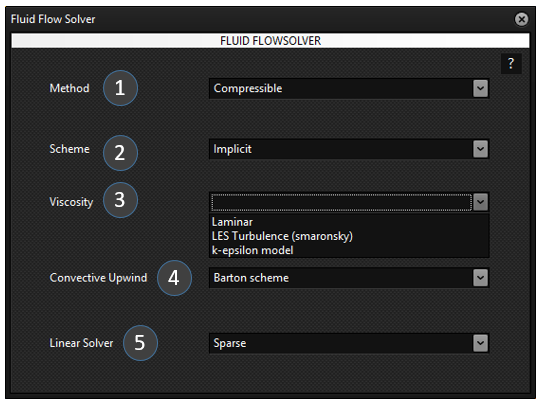
Fig. 7.1: Fluid Flowsolver selection pane for solver setting and its specific schemes.
Description of Fields
1. Method
The Method specifies the governing flow formulation used by the CFD solver.
Available Options
Compressible
The density of the fluid is allowed to vary with pressure and temperature.
Suitable for:
High-speed gas flows
Compressible aerodynamics
Combustion
Shock wave simulations
Pneumatic conveying
Incompressible
The fluid density is assumed to remain constant throughout the simulation.
Suitable for:
Water flow
Oil flow
Low-speed air flow
Mixing tanks
Pipe flow
2. Scheme
The Scheme defines the time integration method used to solve the governing equations.
Available Options
Implicit
The solution at the new time level depends on unknown future values.
Advantages:
Unconditionally stable
Larger time step
Faster convergence for steady-state problems
Preferred for industrial simulations
Explicit
The solution is computed directly from known values at the previous time step.
Advantages:
Simple implementation
Lower memory usage
Limitations:
Requires very small time steps
Stability governed by the CFL condition
3. Viscosity Model
This option specifies the fluid viscosity or turbulence model used during the simulation.
Available Options
Laminar
Assumes smooth, orderly fluid motion without turbulence.
Suitable for:
Low Reynolds number flows
Microfluidics
Creeping flow
Highly viscous fluids
LES Turbulence (Smagorinsky)
Large Eddy Simulation (LES) resolves large turbulent structures while modelling only the smallest eddies using the Smagorinsky sub-grid scale model.
Suitable for:
Transient turbulent flows
Mixing processes
Vortex shedding
Complex industrial flows
Advantages:
High accuracy
Captures transient turbulence structures
Limitations:
Computationally expensive
k-ε Turbulence Model
The k-ε model is a Reynolds-Averaged Navier-Stokes (RANS) turbulence model.
It solves two additional transport equations:
Turbulent kinetic energy (k)
Turbulent dissipation rate (ε)
Suitable for:
General industrial CFD
Pipe flow
Cyclones
Combustion chambers
Mixing tanks
Ventilation systems
Advantages:
Robust
Fast convergence
Widely validated
Moderate computational cost
4. Convective Upwind Scheme
The convective upwind scheme determines how convection terms are discretized during numerical solution.
Available Options
Barton Scheme
The Barton Scheme is a higher-order upwind discretization technique that reduces numerical diffusion while maintaining numerical stability.
Advantages:
Improved solution accuracy
Better prediction of steep gradients
Reduced numerical oscillations
Suitable for convection-dominated flows
Typical applications:
Particle transport
Heat transfer
Species transport
High Peclet number flows
5. Linear Solver
The Linear Solver specifies the numerical algorithm used to solve the linear system of equations generated during each CFD iteration.
Available Options
Sparse Solver
The Sparse Solver is designed for matrices containing a large number of zero elements.
Advantages:
Lower memory consumption
Faster solution for large CFD problems
Efficient for structured and unstructured meshes
Suitable for large-scale industrial simulations
Recommended Settings
Simulation Type
Method
Scheme
Viscosity
Convection
Linear Solver
Water Flow
Incompressible
Implicit
Laminar
Barton Scheme
Sparse
Air Flow
Incompressible
Implicit
k-ε
Barton Scheme
Sparse
Gas Compression
Compressible
Implicit
k-ε
Barton Scheme
Sparse
Fluidized Bed
Compressible
Implicit
LES / k-ε
Barton Scheme
Sparse
Pneumatic Conveying
Compressible
Implicit
k-ε
Barton Scheme
Sparse
Mixing Tank
Incompressible
Implicit
LES
Barton Scheme
Sparse
Working Principle
The Fluid Flow Solver first assembles the governing equations of mass, momentum, energy, and species transport based on the selected physical models. The chosen Method determines whether density variations are considered, while the Scheme controls temporal discretization. The selected Viscosity Model accounts for either laminar or turbulent flow behaviour. The Convective Upwind Scheme defines the numerical treatment of convection terms, and the Linear Solver efficiently solves the resulting sparse algebraic system at every iteration until convergence is achieved.
Notes
Compressible should be selected when density changes due to pressure or temperature are significant.
Incompressible is recommended for most liquid flow simulations.
Implicit schemes generally provide greater numerical stability and permit larger time steps.
Laminar should only be used for low Reynolds number flows where turbulence is absent.
LES offers higher fidelity for transient turbulent structures but requires substantially greater computational resources.
k-ε is the preferred turbulence model for most engineering and industrial CFD applications due to its robustness and computational efficiency.
The Barton Scheme improves accuracy for convection-dominated transport while maintaining stability.
The Sparse Solver is recommended for all large-scale CFD simulations because of its efficient memory usage and faster solution times.
7.2
Setting up:
On the UI upper pane, select ‘Fluid flowsolver’. This gives the selection pane on the left pane to make fluid flowsolver model choices and settings as shown in Fig. 8.1.
The selections include Method (compressible or incompressible), Scheme (implicit or explicit), viscosity (Laminar or any turbulence model), convective upwind scheme and linear solver.
8.
Eulerian Boundary Condition
8.1
Description and theory:
The unstructured grid domain elements consist of cell external faces that may have been designed to have both external and internal boundaries. The boundaries are defined limits of the domain that can have or represent different conditions for the finite domain. Some of the conventional boundary types defined across CAE formats is listed in table 1. Typically in pressure-velocity based CFD solvers the boundary conditions are imposed on pressure, normal and tangential velocities. The table provides the settings for these conditions for various boundaries. The suffix ‘b’ represents the boundary cell condition and suffix ‘c1’ represents the first internal cell to boundary. In case of vector variables normal and tangential direction vector variables are represented as suffix ‘n’ and ‘t’.
Boundary Id
Boundary Name
settings
3
Wall
Pb = Pc1; Ub,n = 0; Ub,t = -Uc1,t;
4
pressure - inlet, inlet - vent, intake – fan
Pb = Pset; Ub,n = eval; Ub,t = Uc1,t;
5
pressure - outlet, exhaust - fan, outlet- vent
Pb = Pset; Ub,n = eval; Ub,t = Uc1,t;
7
Symmetry
-
8
periodic – shadow
-
9
pressure - far - field
Pb = Pc1; Ub,n = eval; Ub,t = Uc1,t;
10
velocity - inlet
Pb = Pc1; Ub,n = Uset; Ub,t = Uc1,t;
12
Periodic
14
fan, porous - jump, radiator
20
mass flow - inlet
Pb = Pc1; Ub,n = mset/ρf; Ub,t = Uc1,t;
24
interface
31
parent(hanging node)
36
Outflow
Pb = Pc1; Ub,n = eval; Ub,t = Uc1,t;
8.2
Setting up:
On the UI upper pane, select ‘Boundary condition’. This gives the selection pane on the left pane to make fluid flowsolver model choices and settings as shown in Fig. 8.1.
The selections include Method (compressible or incompressible), Scheme (implicit or explicit), viscosity (Laminar or any turbulence model), convective upwind scheme and linear solver.
9.
Execute
9.1
Description and theory:
The execute is the final property to be edited before running a simulation. Fig. 9.1 shows the middle pane that is observed on clicking the Execute in the left pane. Here the output settings, time step settings, end time settings and autoload visualization settings are made. The time step size and DEM time step size are related where the DEM time step size needs to be integer greater than 1. The DEM time step here represents the individual time step over which collision particle tracking integration is performed. However, updating of all other forces is performed at the end of time step size only. This is simply because typically in DEM simulations the collision tracking needs to be refined depending on spring dashpot collision time limitations. Therefore, the time step size for other force updation is typically some factor higher than the DEM collision time step size. The other important variable setting is the number of timestep simulation and end time which are both related. Hence they autoset when the other is changed.
9.2
Setting up:
The output path and output time interval needs to be set using the check boxes at the top. The output path is the path where the output data will be written.
Check boxes for time step size, DEM steps/Time step, Number of time step simulations and End time have been provided in the center of the middle pane with the heading ‘Simulation time settings’.
GranDEM Engine Execute
The GranDEM Engine Execute window is the final stage before starting a simulation. It allows the user to define the simulation output location, numerical time settings, execution options, visualization preferences, and monitoring controls. Once all required model settings have been completed, this window is used to execute the DEM or CFD-DEM simulation.
Fig. X.X:GranDEM Engine Execute Window
Field Description
1. Output Path (Write)
Specifies the directory where all simulation output files will be stored.
The generated files may include:
Particle data
Flow field data
Restart files
Log files
ParaView visualization files
Temporary solver files
Use the browse (...) button to select the desired output folder.
2. Output Time Interval (No. of Time Steps)
Defines how frequently simulation results are written to disk.
For example,
Output Interval = 10
means simulation data will be saved every 10 computational time steps.
Smaller intervals produce more output files but require additional storage.
Larger intervals reduce disk usage but provide fewer intermediate results.
Simulation Time Settings
3. Time Step Size (s)
Defines the physical time represented by one computational time step.
Smaller time steps provide
better numerical stability
higher solution accuracy
but require longer computation times.
4. DEM Steps / Time Step
Specifies the number of DEM calculations performed within each CFD time step.
This parameter is mainly used for coupled CFD–DEM simulations.
5. Total Number of Time Steps
Defines the total number of computational iterations performed.
6. End Time (s)
Specifies the total physical duration of the simulation.
The solver automatically terminates once this time is reached.
7. File Name Initial
Defines the filename prefix for all generated simulation files.
Execution Controls
8. Execute
Starts the simulation using all specified settings.
Before execution, ensure that
Geometry has been created.
Materials have been assigned.
Injection conditions are defined.
Force models are selected.
Solver parameters are complete.
Visualization Options
9. ParaView Auto Load
Automatically launches ParaView after completion of the simulation or whenever output files become available.
When enabled, users can immediately visualize
Particle motion
Fluid fields
Velocity vectors
Temperature contours
Pressure distributions
without manually opening ParaView.
10. Restart Switch
Enables simulation restart functionality.
When activated, the solver reads previously saved restart files and continues the simulation from the last saved state instead of beginning from time zero.
This is particularly useful for
long simulations,
interrupted simulations,
extending previously completed analyses.
11. Show Graphical Data
Displays live graphical updates while the simulation is running.
Typical information includes
particle movement,
convergence history,
solver progress,
computational status.
Disabling this option may slightly improve execution speed on slower computers.
Output Management
12. Clear Output
Deletes previously generated simulation output files from the selected output directory.
This option is useful before starting a fresh simulation to avoid mixing old and new result files.
13. Clear Response
Clears the solver response and console messages displayed within the execution window.
Only the displayed log is removed; simulation files remain unchanged.
Solver Response Window
The large console area displays real-time execution messages generated by the solver.
Typical information includes
simulation initialization,
mesh loading,
material loading,
solver progress,
iteration status,
warnings,
numerical errors,
successful completion message.
This console is the primary location for diagnosing simulation problems.
Progress Bar
The progress bar at the bottom of the window indicates the current completion percentage of the simulation.
The progress bar gradually increases until the simulation reaches 100%, indicating successful completion.
Workflow
A typical execution workflow is:
Select the output directory.
Specify the output writing interval.
Define the simulation time step size.
Set the number of DEM steps per CFD time step.
Enter the total simulation time or end time.
Provide a filename prefix.
Enable optional visualization or restart features if required.
Click Execute to start the simulation.
Monitor the solver messages and progress bar until completion.
Visualize the generated results in ParaView or other supported post-processing tools.
Graphical Data – Residual Graph
The Residual Graph tab is used to monitor the convergence of the numerical solution during CFD simulations. A residual represents the error remaining in the governing equations after each solver iteration. As the simulation progresses, these residual values should decrease, indicating that the solution is converging toward a stable state.
Field Description
1. Show Residual Graph
Description: This switch enables or disables the real-time display of the residual convergence graph during the simulation.
Purpose:
Displays the convergence history while the solver is running.
Helps monitor whether the solution is converging properly.
Useful for identifying unstable or diverging simulations.
Options
On – Residual graph is displayed and updated continuously.
Off – Residual graph is hidden.
2. Residual Iterations History
Description: Specifies the number of recent solver iterations to display in the residual graph.
Purpose:
Controls the size of the convergence history shown.
A larger value provides a longer history of convergence.
A smaller value focuses on the most recent iterations.
Typical Value
20
This displays the residual values for the last 20 solver iterations.
Residual Graph
When enabled, the graph typically plots:
Continuity residual
X-Momentum residual
Y-Momentum residual
Z-Momentum residual
Energy residual (if heat transfer is enabled)
Species residuals (if mass transfer is enabled)
The residual values are plotted against the solver iteration number, allowing users to evaluate convergence throughout the simulation.
Interpretation of Residual Graph
Residual Behaviour
Interpretation
Rapid decrease
Good convergence
Slowly decreasing
Stable but slower convergence
Nearly constant
Solution has stagnated
Oscillating
Possible instability
Increasing
Divergence; simulation settings should be checked
Fig. 9.1: The Execute selection from left tab showing the input setting details in the middle pane.
Further, a setup for auto paraview visualisation loading is provided so that the user can get an auto visualization of the data while the simulation is running. This feature can be switched on by the user using the ‘Paraview Auto Load’ switch while setting the autoload timings using the check boxes besides ‘Time Interval’.
In the event of a simulation crash or end of simulation, the user can also restart the simulation directly from where it stopped. This can be done by first switching on the restart switch and setting the time of restart.
10.
FILE, EDIT, SOURCE, FILTERS, AND HELP
10.1
Description and theory:
In the upper left corner of the UI interface is provided with a series of selection for miscellaneous operations and features like FILE, EDIT, SOURCE, etc. The ‘FILE’ selection has options like ‘Open’, ‘Open Mesh File’, ‘Save’, ‘Save As’ and ‘Exit’. The GRANDEM UI ‘Open’ feature can be used to import any standard Grandem case file ‘.gdm’. Similarly, it can also be used to save case ‘.gdm’ file including with password protection. The mesh file can be used to import standard fluent mesh ‘.msh’ file and replace it into the model settings.
Fig 10.1: Selection within ‘FILE’
11.
Paraview Post Processing
11.1
Description and theory:
This selection on the left pane is used after a simulation run has completed and output result data is available for paraview post-processing and visualization study. On selecting this the middle pane appears as shown in Fig. 11.1. Here in this feature various data type files can be loaded into and viewed in paraview. This includes .cgns, .vtk and .cas fluent files for the grid and fluid data while .vtu files for the particle data.
In the middle pane 3 main buttons have been provided to start paraview, reset paraview and delete script. Below this are 4 tabs each having their individual post processing functionalities. The first tab is ‘Grid view’ tab for loading grid and fluid data. The second tab is ‘Particle view’ tab for loading particle data files. The third tab is ‘Multiple View’ tab used for expanding to multiple views of the prevailing view to show velocity field, thermal field and species field.
The Grid View tab is used to visualize the computational mesh (grid) generated for the simulation. It provides options to automatically load the simulation files into ParaView and display the computational domain using different visualization modes.
Grid View is primarily used to inspect the mesh quality, verify imported geometry, and examine internal cross-sections before analyzing simulation results.
Fig. 11.1: ParaView AutoScript – Grid View
Field Description
1. Run ParaView
Launches ParaView automatically and executes the generated visualization script. The selected simulation files are loaded without requiring manual import.
2. Reset ParaView
Resets the current ParaView visualization to its default state. Previously loaded objects, filters, and display settings are removed.
3. Delete Script
Deletes the automatically generated ParaView Python script. A new script will be generated the next time visualization is requested.
4. Grid View
Displays the computational mesh (grid) of the simulation domain. This view is mainly used to inspect the generated mesh and geometry before viewing particle or flow results.
5. Particle View
Switches to the particle visualization interface where Lagrangian particles can be displayed and analyzed.
6. Multiple View
Opens multiple visualization windows simultaneously, allowing different datasets or viewpoints to be observed together.
7. Save
Saves the current visualization configuration, including selected options and display settings, for future use.
8. Load CGNS
Loads simulation results stored in the CGNS (CFD General Notation System) format into ParaView.
Typical use:
Structured CFD datasets
Flow field visualization
Pressure, velocity and temperature contours
9. Load VTK
Loads simulation data stored in the VTK (Visualization Toolkit) format.
This format is commonly used for:
DEM particle results
Volume data
Surface meshes
Scalar and vector fields
10. Load CAS
Loads Fluent mesh or case files (.cas) into ParaView for visualization.
This option is useful when GranDEM is coupled with ANSYS Fluent or when Fluent-generated meshes need to be inspected.
11. 3D View
Enables full three-dimensional visualization of the computational grid.
When enabled, the complete geometry is rendered in 3D, allowing the model to be rotated, zoomed, and inspected from any viewing angle.
12. Opacity (3D View)
Controls the transparency of the 3D computational mesh.
0 → Completely transparent
1 → Completely opaque
Lower opacity values allow internal regions of the mesh to become visible.
13. Slice View
Displays a two-dimensional cross-sectional slice through the computational domain.
Slice View is useful for examining:
Internal mesh quality
Pressure distribution
Velocity contours
Temperature fields
Concentration profiles
without hiding the interior of the model.
14. Opacity (Slice View)
Controls the transparency of the slice plane displayed in ParaView.
Increasing opacity makes the slice easier to observe, while lower values allow the surrounding geometry to remain visible.
15. Normal Direction (X, Y, Z)
Defines the orientation of the slicing plane.
The slice plane is positioned perpendicular to the specified normal vector.
Examples:
(1, 0, 0) → Slice normal to the X-axis (YZ Plane)
(0, 1, 0) → Slice normal to the Y-axis (XZ Plane)
(0, 0, 1) → Slice normal to the Z-axis (XY Plane)
Custom vector values can also be specified to create slices at arbitrary orientations.
Working Procedure
Open ParaView AutoScript → Grid View.
Choose the desired simulation file format (CGNS, VTK, or CAS).
Enable 3D View to visualize the complete computational mesh.
Adjust the Opacity to inspect internal mesh regions if required.
Enable Slice View to create a cross-sectional view of the model.
Specify the Normal Direction (X, Y, Z) to define the orientation of the slice.
Click Run ParaView to automatically launch ParaView and load the selected dataset.
Particle View
The Particle View tab in the ParaView AutoScript module is used to visualize DEM particle results generated during a GranDEM simulation. It provides two methods for loading particle data depending on how the simulation results are stored.
Fig. 11.2: ParaView AutoScript – Particle View
Fields Description
1. Load VTU Data (using PVD)
Description: Loads particle data using a PVD (ParaView Data Collection) file. The PVD file references all VTU files generated during the simulation and automatically organizes them into a time series.
Purpose:
Loads all simulation time steps at once.
Enables animation of particle motion.
Automatically updates the timeline in ParaView.
Recommended for transient simulations with multiple output files.
Typical Use:
Use this option after completing a simulation when multiple VTU files have been generated for different time steps.
2. Load VTU Data (Direct)
Description: Loads an individual VTU (VTK Unstructured Grid) file directly into ParaView without requiring a PVD file.
Purpose:
Opens a single simulation result.
Useful for inspecting one specific time step.
Faster when only one output file needs to be visualized.
Suitable for debugging or post-processing individual datasets.
Typical Use:
Use this option when viewing a single VTU file or when a PVD file is not available.
Recommended Workflow
Run the DEM simulation in GranDEM.
Generate particle output files (VTU/PVD).
Open ParaView → Particle View.
Select one of the following options:
Load VTU Data (using PVD) for complete time-dependent visualization.
Load VTU Data (Direct) for viewing a single particle dataset.
Analyze particle trajectories, distribution, velocity, collisions, and other DEM results in ParaView.
Multiple View
The Multiple View tab allows users to create multiple visualization windows in ParaView simultaneously. This feature enables different simulation variables to be displayed side-by-side, making it easier to compare flow behavior, temperature distribution, and species concentration within the same simulation.
Multiple View is particularly useful during post-processing when several physical phenomena need to be analyzed together.
Fig. 11.3: ParaView AutoScript – Multiple View
Field Description
1. Create Multiple Views
Description: Creates multiple synchronized visualization windows in ParaView.
Purpose:
Displays several simulation results simultaneously.
Allows comparison of different physical quantities.
Improves post-processing efficiency.
Eliminates the need to repeatedly switch between variables.
Typical Usage:
After selecting the desired visualization options, click Create Multiple Views to automatically generate the corresponding ParaView layout.
2. Velocity Field View
Description: Enables visualization of the fluid velocity field.
Purpose:
Displays:
Velocity magnitude
Velocity vectors
Flow direction
Flow patterns
Recirculation zones
Vortices
Applications:
Fluid flow analysis
CFD verification
Mixing studies
Pneumatic conveying simulations
Particle-fluid interaction analysis
3. Thermal View
Description: Enables visualization of temperature distribution within the simulation domain.
Purpose:
Displays:
Temperature contours
Thermal gradients
Heat transfer regions
Hot spots
Cooling zones
Applications:
Heat transfer simulations
Drying processes
Combustion analysis
Thermal management studies
CFD-DEM heat transfer investigations
4. Species View
Description: Enables visualization of species concentration or mass fraction distribution.
Purpose:
Displays:
Species concentration contours
Mass fraction distribution
Diffusion behavior
Mixing characteristics
Mass transfer regions
Applications:
Multicomponent flow simulations
Gas-solid reactions
Drying processes
Evaporation studies
Chemical transport simulations
Working Procedure
Open ParaView → Multiple View.
Enable one or more visualization options:
Velocity Field View
Thermal View
Species View
Click Create Multiple Views.
ParaView automatically generates separate synchronized windows.
Rotate, zoom, and inspect results simultaneously across all selected views.
Advantages of Multiple View
Simultaneous comparison of multiple variables.
Faster interpretation of simulation results.
Better understanding of coupled physical phenomena.
Useful for CFD, DEM, and CFD-DEM simulations.
Supports advanced engineering analysis and reporting.
Example
For a CFD-DEM drying simulation:
View
Variable Displayed
Velocity Field View
Air velocity distribution
Thermal View
Temperature distribution
Species View
Moisture concentration distribution
This allows the engineer to observe how airflow affects heat transfer and moisture removal at the same time.
Save
The Save tab of the ParaView AutoScript module provides options for exporting simulation visualizations and managing camera positions. It allows users to save animations of transient simulations and store predefined camera orientations for consistent visualization and reporting.
Fig. 11.3: ParaView AutoScript – Save View
Field Description
1. Save Animation
Description: Exports the currently loaded simulation as an animation file using the visualization settings defined in ParaView.
Purpose:
Creates an animation of the simulation.
Captures particle movement and fluid flow over time.
Generates presentation-quality videos.
Useful for reports, publications, and demonstrations.
Output
Typical output formats include:
AVI
MP4
Image sequence (PNG/JPEG)
(depending on the ParaView export configuration)
2. Frame Rate
Description: Specifies the number of animation frames displayed per second (FPS).
Purpose:
Controls the playback speed of the exported animation.
Higher frame rates produce smoother animations.
Lower frame rates create slower playback.
Typical Values
Frame Rate
Usage
1 FPS
Slow scientific visualization
10 FPS
General simulation playback
24 FPS
Standard video
30 FPS
Smooth animation
60 FPS
High-quality visualization
Camera Angles
The Camera Angles section allows users to save and reuse predefined camera positions for consistent visualization.
3. Camera Angle Selection
Description: Displays a list of previously saved camera positions.
Purpose:
Select an existing camera orientation.
Reuse the same viewing angle across different simulations.
Maintain consistent figures for reports and publications.
4. Get
Description: Retrieves the currently selected camera angle from the list.
Purpose:
Loads the saved camera parameters.
Prepares the selected view for application.
5. Save Camera Angles
Description: Stores the current ParaView camera position and orientation.
Purpose:
Saves camera location.
Saves viewing direction.
Saves zoom level.
Saves focal point.
This allows the same viewpoint to be reused later.
6. Apply Camera Angles
Description: Applies the selected saved camera angle to the current visualization.
Purpose:
Restores a previously saved viewpoint.
Ensures identical viewing orientation across multiple simulations.
Produces consistent screenshots and animations.
Working Procedure
Open ParaView → Save.
Adjust the visualization to the desired viewpoint.
Click Save Camera Angles to store the current camera position.
Select the desired Frame Rate for animation playback.
Click Save Animation to export the simulation.
For future simulations, choose a saved camera angle and click Apply Camera Angles to reproduce the same visualization.
Advantages
Generates high-quality simulation animations.
Produces consistent camera views across different projects.
Simplifies report and presentation preparation.
Reduces manual adjustment of camera orientation.
Improves reproducibility of visualization results.
11.2
Setting up:
Check if paraview has been started. If not start paraview by clicking the button ‘Run Paraview’.
The first tab ‘Grid view’ can be seen in Fig. 9.1 where 3 buttons have been provided to load either vtk, cgns or cas files. By selecting the check box ‘3D view’ and/or ‘Slice view’ Opacity and slice plane direction can be set before loading.
When any of the ‘load’ button is clicked a selection dialog box opens to browse to the folder that contains the data files. Browse to the location folder and select the folder to press ok. This loads the data files into paraview.
Move to the ‘Particle View’ tab where on clicking Load VTU button a dialog box opens to browse the data folder location. Browse to the data file location where .pvd file can be located. Select the .pvd file and click ‘open’. This loads particle data files.
The next tab is ‘Multiple view’ tab that is utilized when multiple view are to be created simultaneously. This tab has the button ‘Create Multiple views’ (Fig. 9.2) that on clicking creates 4 render views.
This tab further has check boxes for ‘velocity field view’, ‘thermal view’ and ‘species view’ all of which can be selected based on user requirement. The ‘Apply view’ button sets up the parallel views of the selected views in the check boxes.
The ‘Save’ tab has the functionality to save animations after setting frame rate for the video as show in Fig. 9.3. Besides, this tab also has camera angles saving functionality that sets and saves camera view angles with specific names by clicking the ‘Save Camera Angles’ button.
The saved camera angles can be used to select from the drop down menu. When the ‘Apply Camera Angles’ button is used the selected camera angle view is shown or presented. This button can be used for resetting back to a specific angle that the user wants to set.
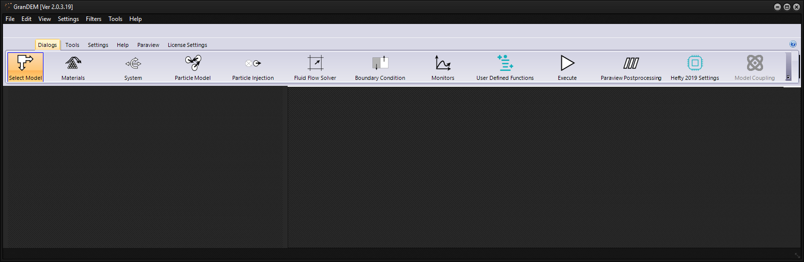
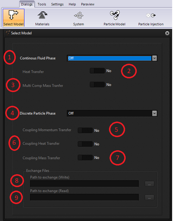
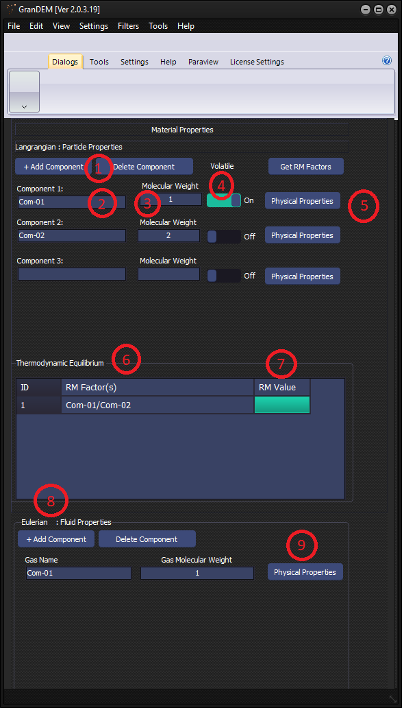
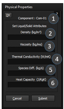
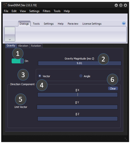
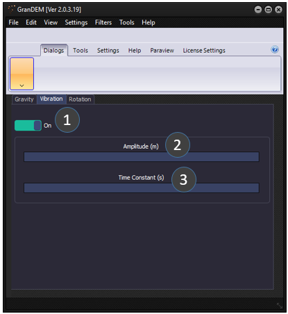
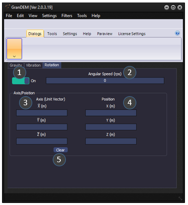
 (3.1)
(3.1)
 (3.2)
(3.2) (3.3)
(3.3) (3.4)
(3.4) (3.5)
(3.5) (3.6)
(3.6)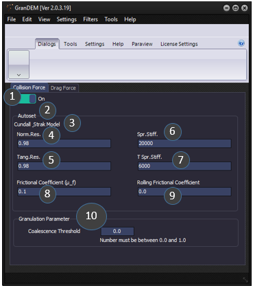
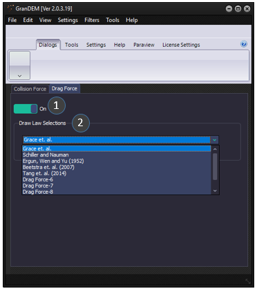
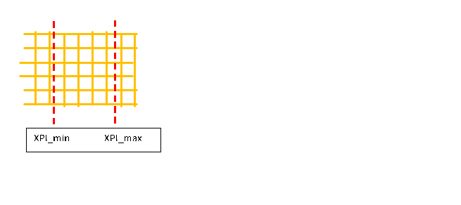
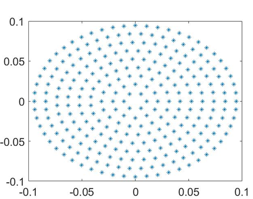
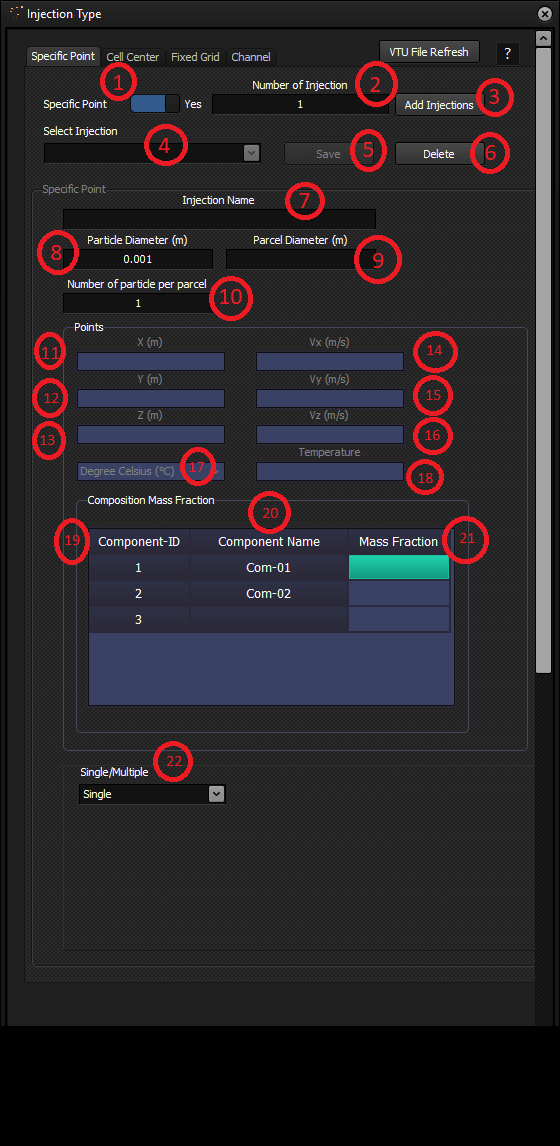
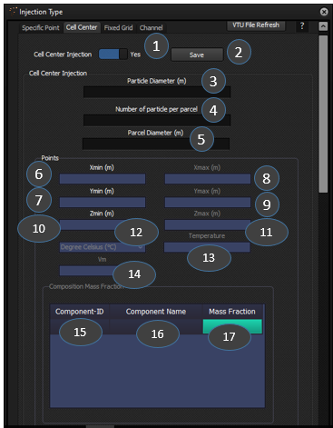
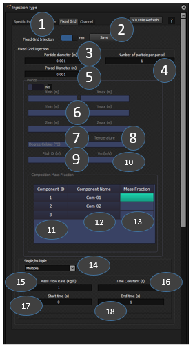
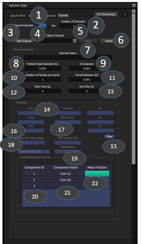
 (8.1)
(8.1) (8.2)
(8.2) (8.3)
(8.3) (8.4)
(8.4) (8.5)
(8.5) (8.6)
(8.6) (8.7)
(8.7) (8.1)
(8.1) (8.4)
(8.4) (8.7)
(8.7)